Often when faced with an unsatisfactory binary choice, the best solution may be to go a third way. In this context, it could be the so-called "hybrid model", which delivers the validity advantages of the fixed-effects model with the parsimony (and thus precision) advantages of the random effects model. There are ways that this model can go wrong, too, but in many situations, you can have your cake and eat it, too. Presenting this result to a Francophone audience last year, I learned that the way to express that latter sentiment is that you can have both the butter and the butter money.
|
Some of my best friends are fixed-effects Nazis, but I have long been worried about the potential loss of power in situations where there are relatively few observations per cluster and fixed effects drop out all of the concordant strata. You might gain some validity, but at the price of precision, and therefore do worse in terms of MSE. Now I see a new paper that finally addresses this trade-off in greater detail. The Hausman test is treated with great reverence in some quarters, but it is a significance test, after all, and so has all of the usual weaknesses of significance testing, such as the potential for low power to correctly reject the null in some settings, or excessive power to reject a trivially false null in other situations.
Often when faced with an unsatisfactory binary choice, the best solution may be to go a third way. In this context, it could be the so-called "hybrid model", which delivers the validity advantages of the fixed-effects model with the parsimony (and thus precision) advantages of the random effects model. There are ways that this model can go wrong, too, but in many situations, you can have your cake and eat it, too. Presenting this result to a Francophone audience last year, I learned that the way to express that latter sentiment is that you can have both the butter and the butter money.
3 Comments
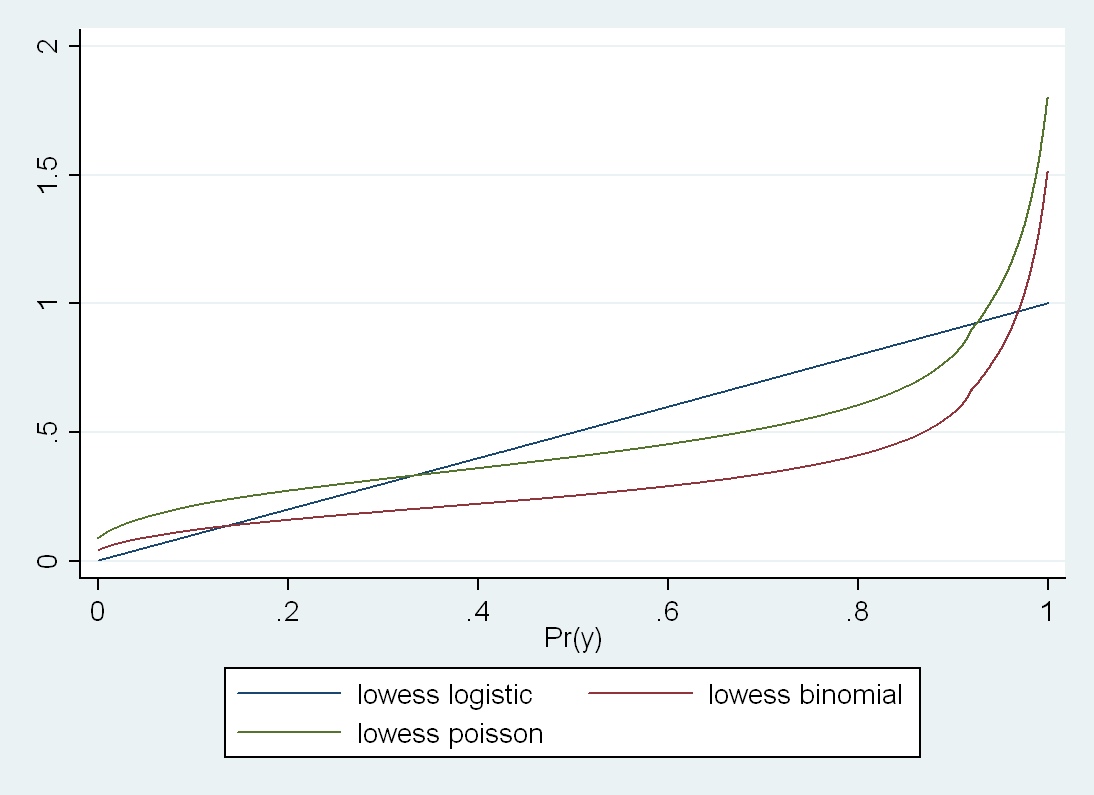
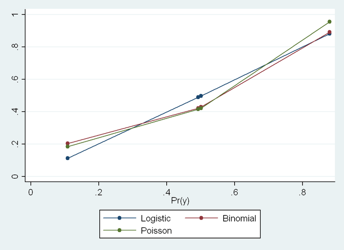 We all know that the change in estimate approach to finding confounders can't work for the OR because the OR can change its value when conditioned on any determinant of outcome, even if the covariate is independent of exposure. Therefore, the OR will "cry-wolf" and claim confounders that aren't confounders (when they are not associated with exposure). It can also fail to detect a true confounder, although a recent paper by Mansournia and Greenland notes that this is decidedly less likely to occur, because it requires an incidental canceling out. On the other hand, the false accusation of confounders by a change in estimate approach applied to an OR is quite easy to encounter. This will happen whenever the frequency of the outcome is high in the data set. Here is a quick Stata example that generates a data set of binary variables: clear all set obs 10000 set seed 12345 gen c = rnormal() gen x = rnormal() gen y = rnormal() + x + c replace c = (c > 0) replace x = (x > 0) replace y = (y > 0) This code generates a binary Y that is a function of both exposure X and covariate C. X and C are completely independent (ORXC = 1). Therefore C by definition cannot be a confounder. Prevalence of Y=1 is 0.5. logistic y x logistic y x c Crude ORYX = 5 When I adjust this for C, I get ORYX|C = 7. Therefore, by change in estimate criteria, one might think that they have to adjust for C. But this is wrong. The OR is "crying wolf". So far so good. We also know that the RD is collapsible, and sure enough: binreg y x, rd binreg y x c, rd Crude RDYX = 0.38 When I adjust this for C, I get RDYX|C = 0.38. Therefore, by change in estimate criteria, one would not adjust for C, which is the right answer. Good. But here is the surprise: binreg y x, rr binreg y x c, rr Crude RRYX = 2.30 When I adjust this for C, I get RRYX|C = 2.08. These are significantly different, and therefore, by change in estimate criteria, one might adjust for C, which would be a mistake. The RR is supposed to be collapsible, so this baffled me until I looked at the stratum specific estimates: cs y x, by(c) cs y x, by(c) istandard cs y x, by(c) estandard c | RR [95% CI] -----------------+------------------------------------- 0 | 4.54 4.04, 5.11 1 | 1.75 1.68, 1.83 -----------------+------------------------------------- Crude | 2.30 2.19, 2.40 M-H combined | 2.26 2.16, 2.36 I. Standardized | 2.24 2.15, 2.34 E. Standardized | 2.27 2.18, 2.37 For those of you who don't know Stata, "internally standardized" is standardization using the X=1 group as the target population, and "externally standardized" is standardization using the X=0 group as the target population (old occupational health terminology). X and C are uncorrelated in expectation, so these target-population-specific adjusted values differ only due to the chance imbalance in C across levels of X. So there is tremendous effect modification by C here, even though C is not a confounder. This doesn't seem to matter for the RD, but for the RR, getting the right answer seems to depend on exactly HOW I adjust for C. These standardized estimates are slightly different, but they are all statistically homogeneous with the crude. But the binomial regression adjusted estimate is much lower than the standardized estimates (RR = 2.09). If I use Poisson regression, I get RR=2.26, so again it is collapsible, so it seems that only the binomial regression estimate is screwy here. Should one avoid binomial regression when the outcome is common or the effect of the exposure is heterogeneous? I was sincerely confused, so I sent e-mail around to some friends, and after some discussion, it all seemed quite obvious. My Stata code generates the following (true) proportions of Y=1 in each stratum of X and C: . table x c, c(mean y) ------------------------------ | c x | 0 1 ----------+------------------- 0 | 0.1084666 0.5012356 1 | 0.4927478 0.8789078 ------------------------------ Logistic regression: ------------------------------ | c x | 0 1 ----------+------------------- 0 | 0.112023 0.4974815 1 | 0.4890754 0.8825148 ------------------------------ Binomial regression: ------------------------------ | c x | 0 1 ----------+------------------- 0 | 0.2031814 0.4296737 1 | 0.4217731 0.8919361 ------------------------------ Poisson regression: ------------------------------ | c x | 0 1 ----------+------------------- 0 | 0.1835052 0.4220249 1 | 0.4152605 0.9550153 ------------------------------ Logistic is not perfect here, but much better than the other two. Still, it is not that logistic is somehow superior in any general sense for this task. It just got lucky in this instance. The two stratum-specific ORs are 8.0 and 7.2, which happen to be much closer to being homogeneous than the two true RR’s (4.5 and 1.8). The fact that the two true RDs are roughly homogeneous (0.38 and 0.38) explains why the additive model does so well. As Rich MacLehose kindly pointed out, this has nothing to do with collapsibility, per se. It has to do with model fit. If the model is misspecified, you can easily get change in estimate that suggests confounding, regardless of the choice of effect estimate. In *ALL* of these models, when I add an interaction term, I get the exactly correct predicted proportions in every cell, and the correct RRs or ORs when I divide these predictions. So the moral of the story is that change in estimate is not a sufficient criterion, even with a collapsible measure. One also has to get the model right. Seems obvious in retrospect, but in practice, how often do we worry about this? The well-known Greenland and Morgenstern example shows RR collapsibility even when the stratum specific RRs are very heterogeneous, but they use tabular (i.e. non-parametric) adjustments In their example, if one used a regression model, one would not generally reach the same conclusion (without adding interaction terms). But Rich also asked another question, which is how it can be that Poisson Regression and Binomial Regression produce different point estimates when they have the same link function and differ only in the error distribution. I also hadn't previously thought in detail about this, and if students asked I probably would have answered the same: that changing the distribution in the GLM would affect the CIs but not the point estimates. But I think that my (bad) intuition stems from equating rates and risks. If the outcome were rare, I think we would indeed see that these give approximately the same value. But the problem is that the outcome in my example is common, and in some cells VERY common. That apparently messes things up. Specifically, logistic model searches for the best (ML) solution under the constraint that all the log-odds fall on a straight line. Binomial regression searches for the best (ML) solution under the constraint that all the log-risks fall on a straight line. Poisson searches for the best (ML) solution under the constraint that all the log-rates fall on a straight line. So I guess what we are seeing here is the distinction between risks and rates. The surprising thing about that is that I have no person time here (no offset in the Poisson model), so everyone has 1 time unit, so I can't see how the rate and risk could be different. So that remains a bit of a mystery for me. If you look at a plot of the fitted values for the three models (truth versus logistic, binomial and Poisson), you see that logistic comes closest in this instance because the true proportions are closest to being linear in the log odds than to any of the other scales: But even though Binomial and Poisson match almost exactly on the low end, they diverge markedly at the high end. This makes me think that we could see the distinction much more clearly if we don't convert everything to binary variables. So I ran this again with continuous x and c: I had a hard time getting binomial regression to converge, and ended up having to plot this with a smoother because the predicted line was jagged for binomial because of the difficulty in obtaining convergence. But in any case, now one can see that the shape of the underlying function is rather different between Poisson and Binomial here. If you don't smooth, Poisson shoots up
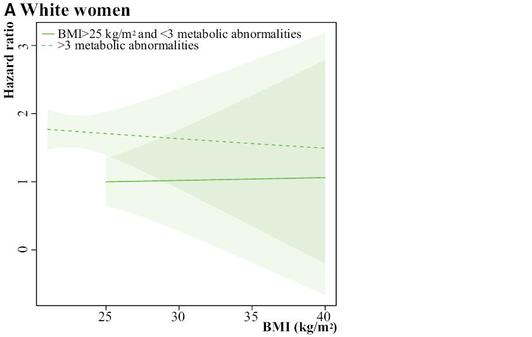
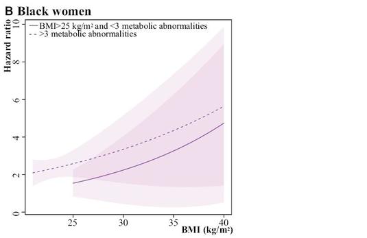
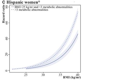
much more dramatically at the upper limit as you get very close to 1 in the true probability. Even on the low end they are not that close, but I think that this is because the model is trying to find the ML solution that also works on the top end. And bear in mind that the logistic looks straight here only because the data in my particular example happened to be approximately homogeneous in the ORs across strata of C, but one could engineer an example where logistic would do very poorly, too. Moral of the story: use interaction terms to make a saturated model, and then use –margins- to take the differences or ratios of the correctly specified risks (what Sam Harper recommended to me from the start). Common wisdom that Poisson and Binomial are estimating the same parameter comes from a rare outcome setting. When the outcome is not rare, these are not going to agree, and there is no way to predict which will be closer to the truth in any given instance. Again, all this seems obvious in retrospect, but then again, most things do. 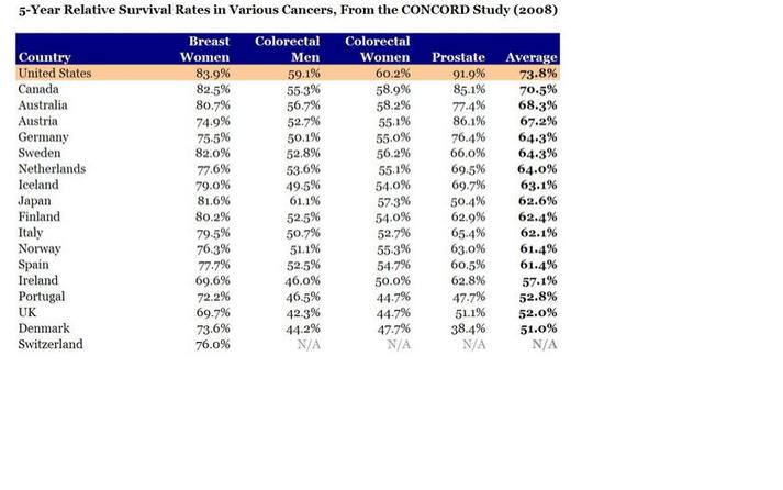 In this new paper, Chris Murray's team at the Institute for Health Metrics and Evaluation reports on mortality, incidence, years lived with disability (YLDs), years of life lost (YLLs), and disability-adjusted life-years (DALYs) for 28 cancers in 188 countries by sex from 1990 to 2013. The only problem is that perhaps three-quarters of those 188 countries produce no meaningful data whatsoever on these quantities. But the figures and graphs are stunningly beautiful. But with even mortality data so unreliable in most of the world, why go the extra strep and try to report cancer incidence? Clearly Murray’s professional strategy for getting money and attention is claiming to know everything, or at least being able to provide a number for everything. Thus, it would not serve him to publish something more restrained or conservative. Others could do that, but his unique forte is the chutzpah to assign a number EVERYWHERE for EVERYTHING. And he also knows that he will never be held accountable for these numbers, so what does it matter to him if he is off by a factor of 2 or even a factor of 10? His strategy is wildly successful, especially with powerful benefactors such as Bill Gates and Richard Horton. In short, his fantastic success is due to publishing papers that overreach, just like this one. But surely the issue of cancer incidence is more complicated because any country that screens more will find more cancers, and will therefore also lengthen the time that people spend with cancer and the number of people who ultimately die with cancer (even if not from cancer). So you can get data like these: How does the US, which does not have the highest life expectancy by any stretch, have the highest 5-year survival for every cancer on this table? By aggressive screening of old people for a profit, which I assume is not a characteristic of the health system of any other country shown. For example, Switzerland had a 2012 age-standardized cancer mortality rate for women of 83.9/100,000, whereas for the US it was 104.2/100,000. How does the US have such a high percentage of women surviving 5 years with breast cancer but at the same time, 20% more eventually dying of breast cancer? It has to be via finding smaller tumors sooner. In poor countries, you can have lower incidence (because of less screening) and thus lower mortality from cancer, even in the context of higher mortality overall. Therefore, lowering one’s national cancer incidence and mortality rates can hardly be taken to be a sign of success. I therefore can’t see any value to this surveillance activity for incidence, driven as it is by arbitrary policies on case finding that don’t necessarily benefit patients in terms of costs or longevity. I think we only want to know overall life expectancy, or perhaps quality adjusted or disability adjusted survival. But not cause specific incidence. Maybe not even cause specific mortality. Certainly not for a disease like cancer that is subject to so much arbitrariness in the timing of case ascertainment. Arnaud Chiolero adds: I agree that 5 years survival cannot be used for the surveillance of cancer (see here). The incidence is also misleading for many cancers (e.g., breast cancer in the US), but not for all (incidence of lung cancer is coherent with smoking trends, at least for the moment; it will change when screening becomes more frequent). However, mortality rates are much less biased and trying to measure and reduce cancer mortality rates is a reasonable goal, I think (see here). An author with the delightfully sonorous surname "Schmiegelow" has published a paper in The Journal of the American Heart Association on the relation between obesity, metabolic abnormalities and increased CVD risk across various ethnic/racial groups of post-menopausal women in the WHI data. The authors use Cox models to estimate associations between risk factors and first CVD events over 13 years of follow-up. The results suggest some heterogeneity in the impact of BMI by race among those with no metabolic syndrome: Among black women without metabolic syndrome, overweight was still associated with outcomes (HR=1.49), but not among white women without metabolic syndrome (HR=0.92, heterogeneity p-value 0.05). Likewise for obesity in the absence of metabolic syndrome, black women had a stronger relationship than white women (HR=1.95 versus HR=1.07, heterogeneity p-value = 0.02). Finally, overweight and obese women with ≤1 metabolic abnormality did not have increased CVD risk in any racial category, supporting the "fat but fit" hypothesis. This is all fine, but my question is: what is up with Figure 5? The legend says: "The shaded regions around the lines gives [sic] the 95% confidence band, the standard error, for the mean." I don't really understand that sentence, grammatically. The authors then write: "Please note that the scale of the y-axis differs for white (0 to 3), black (0 to 10), and Hispanic (0 to 80) women, so the widths of the CIs are not comparable." First of all, how can the Hispanic women with BMI=40 have an HR=80? That is a bit suspicious, to say the least. Then, about the confidence interval widths, I get that the vertical scale is different, but nonetheless:
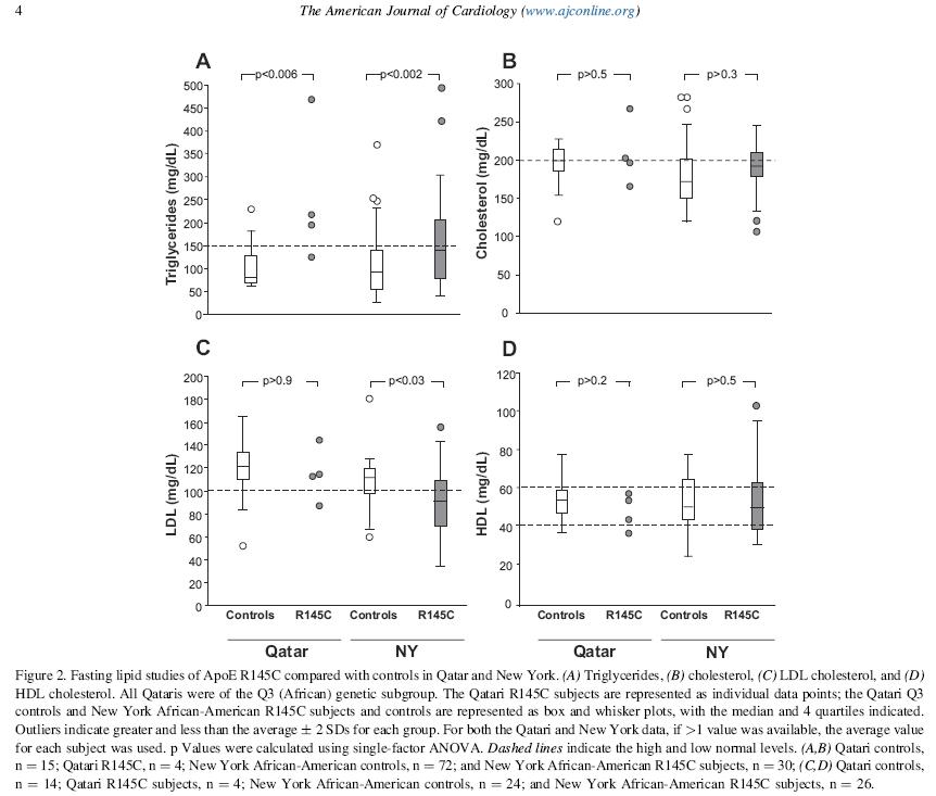
For black women at BMI = 40 and > 3 abnormalities, HR = 5, 95% CI = 1,10 (10 fold wide) For Hispanic women at BMI = 40 and > 3 abnormalities, HR = 75, 95% CI = 70,80 (1.5 fold wide) So Hispanic women are about 10x more precise, despite being the smallest group in the study (6700 whites, 5100 blacks, and 2500 Hispanics). Could this be the first hint that the WHI data are all completely fabricated? The history of genetics is the history of promises. This statement is attributed to historian Nathaniel Comfort in a recent diatribe by David Dobbs, which was posted at Buzzfeed. The delightfully pessimistic Dobbs essay is especially hard on genetic testing, which took a further beating this week in the New England Journal of Medicine when it was reported that different laboratories offer wildly different interpretations of the same genetic tests. There seems to be a consensus around the notion that most genetic testing for predisposition to common diseases is "not ready for prime time", and yet the tsunami of false positive claims continues in the literature unabated, and each time with recommendations for more population screening. This press release reports on a 2013 study by Ziki et al in the American Journal of Cardiology, which describes a genetic variation that is linked to increased levels of triglycerides, and which the authors assert is more common than previously believed and disproportionately affects people of African ancestry. "The finding offers a clue as to why Africans and people of African descent have an increased risk of cardiovascular disease and type 2 diabetes compared to many other populations, says the study's senior author, Dr. Ronald Crystal, chairman of genetic medicine at Weill Cornell. African Americans with the variant had, on average, 52 percent higher triglyceride levels compared with blacks in the study who did not have the variant." But have a look at Figure 2 from Ziki et al: You can immediately see that the whiz-bang result here is actually due to one or two outliers in Panel A. In the Qatar sample in panel A, there is one individual with the mutation who has high triglycerides. In the NY sample in Panel A, the distribution in the affected individuals is shifted up a bit, but is completely overlapping, except for 2 individuals. When your major new result rests on 1 or 2 individuals in each location, there is probably some basis to worry about over-interpretation. Especially because there are also outliers in the control group. And yet the authors imply (last paragraph of the discussion section) that we should now do population screening for this variant.
OK, this is a rather juvenile sentiment to express, but I have to confess that I love Wikipedia. The other day I was looking up information on pre-Capernican systems for explaining observed planetary motion, and came across the remarkable entry for Tycho Brahe. Brahe was a noseless 16th Century Danish nobleman known for important contributions to alchemy and the mechanics of an earth-centered solar system, none of which turned out to be even vaguely correct, of course. So first, there is the nose issue. Wikipedia explains that while studying in the German city of Rostock in 1566, Tycho lost his nose in a duel, the dispute arising with his cousin over the veracity of a mathematical formula. As neither gentleman was sufficiently mathematically equipped to prove his opinion on the matter, they decided to have a duel in order to settle the argument. In the dark. If more math controversies were resolved in this way, think of the epidemic of noselessness that might befall university math departments! "For the rest of his life, he was said to have worn a replacement made of silver and gold, using a paste or glue to keep it attached", explains Wikipedia, along with a photo of a nose similar to that which Tycho wore (but not Tycho's actual nose):  The other issue of interest is Tycho's Elk. Wikipedia cites someone named Pierre Gassendi to the effect that Tycho kept a domesticated elk in his castle. The text then explains:
"[H]is mentor the Landgrave Wilhelm of Hesse-Kassel (Hesse-Cassel) asked whether there was an animal faster than a deer. Tycho replied, writing that there was none, but he could send his tame elk. When Wilhelm replied he would accept one in exchange for a horse, Tycho replied with the sad news that the elk had just died on a visit to entertain a nobleman at Landskrona. Apparently during dinner the elk had drunk a lot of beer, fallen down the stairs, and died." There is no accompanying photo of an elk, similar to the kind owned by Tycho, but not his actual elk. If one's research question is: "Does X have a causal effect on Y?", there are some obvious questions that one would ask before interpreting an observed association causally. For example, "Is there something unmeasured that affects both X and Y?". Among the most obvious of these preliminary questions is: "Does Y in fact cause X?" This would be especially salient in a cross-sectional study, which is why there is so much emphasis put on the term "prospective" in reporting designs that are NOT cross-sectional.
So if that is so painfully obvious that it would be embarassing to even mention it again, why does one read reports like this one on a daily basis? The headline is: Obese teens' brains unusually susceptible to food commercials, study finds and the summary text below the headline is: TV food commercials disproportionately stimulate the brains of overweight teenagers, including the regions that control pleasure, taste and -- most surprisingly -- the mouth, suggesting they mentally simulate unhealthy eating habits that make it difficult to lose weight later in life. The study conducted fMRI exams on 40 right-handed adolescents, 20 normal weight and 20 obese, so everything is cross-sectional. The discussion reveals an interpretation clearly in the causal direction that being obese makes your brain more susceptible to food commercials: Collectively, these findings suggest that higher-adiposity adolescents more strongly recruit oral somatomotor and gustatory regions pertinent to eating behaviors while viewing food commercials, in comparison with their lower-adiposity counterparts. How is it that none of these study authors with doctoral degrees seems to have ever wondered how these children got to be obese in the first place? Writing in the New York Review of Books, Jeremy Waldron has a nice take-down of "nudging", the new buzzword for paternalistically tilting behavior for the good of the individual and/or society.
Waldron has some great paragraphs on knowledge translation in public health, which warrant wider reading and some thinking about why we disseminate information in the way that we do: "[B]etween 15 and 20 percent of regular smokers (let’s say men sixty years old, who have smoked a pack a day for forty years) will die of lung cancer. But regulators don’t publicize that number, even though it ought to frighten people away from smoking, because they figure that some smokers may irrationally take shelter in the complementary statistic of the 80–85 percent of smokers who will not die of lung cancer. So instead they say that smoking raises the chances of getting lung cancer. That will nudge many people toward the right behavior, even though it doesn’t in itself provide an assessment of how dangerous smoking actually is (at least not without a baseline percentage of nonsmokers who get cancer). Or consider the way lawmakers nudge people away from drunk driving. There are about 112 million self-reported episodes of alcohol-impaired driving among adults in the US each year. Yet in 2010, the number of people who were killed in alcohol-impaired driving crashes (10,228) was an order of magnitude lower than that, i.e., almost one ten thousandth of the number of incidents of DWI. The lawmakers don’t say that 0.009 percent of drunk drivers cause fatal accidents (implying, correctly, that 99.991 percent of drunk drivers do not). They say instead that alcohol is responsible for nearly one third (31 percent) of all traffic-related deaths in the United States—which nudges people in the right direction, even though in itself it tells us next to nothing about how dangerous drunk driving is. There’s a sense underlying such thinking that my capacities for thought and for figuring things out are not really being taken seriously for what they are: a part of my self. What matters above all for the use of these nudges is appropriate behavior, and the authorities should try to elicit it by whatever informational nudge is effective. We manipulate things so that we get what would be the rational response to true information by presenting information that strictly speaking is not relevant to the decision.... ...[I]t helps us see that any nudging can have a slightly demeaning or manipulative character. Would the concern be mitigated if we insisted that nudgees must always be told what’s going on? Perhaps. As long as all the facts are in principle available, as long as it is possible to find out what the nudger’s strategies are, maybe there is less of an affront to self-respect. Sunstein says he is committed to transparency, but he does acknowledge that some nudges have to operate “behind the back” of the chooser." Our paper (first-authored by Britt McKinnon) sat at Maternal Child Health Journal for almost 6 months, and came back today as "revise and resubmit" with 6 reviews, but each one was only a few lines long.
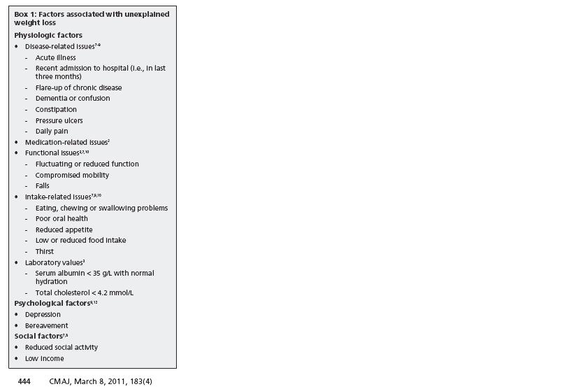
For example, Reviewer 3 had only 3 lines of comments, which were numbered 1), 2) and 2). The second comment number 2 was: "The use of word WE is repeated so many times. Please change it at least in a few places to enhance readability." to which we intend to repond: "We agree." But the best comment of all time goes to reviewer 5, who states (with no apparent irony or embarassment): "The paper is very statistically oriented and would do well with a more ideological approach." In this new article, Dowd and Zajacova consider the question of cumulative dose of obesity over the lifecourse, and how this might impact on later life functional disabilities. They analysed data from over 7000 adults ages 60–79 from the 1999–2010 NHANES survey, with the outcome being a self-report of difficulty or severe difficulty with any of eight functional tasks. The exposure was self-reported 25-year old BMI (does anyone really know that?). Predictably, there was an association between 25-year-old obesity (BMI > 30 kg/m2) and functional limitations, and this was greatly diminished in magnitude after controlling for current BMI. For severe limitations, for example, the covariate-adjusted OR for age 25 obesity was 2.72 (95% CI: 2.13–3.46), and this diminished to 1.32 (95% CI:1.00–1.75) after adjustment for current BMI. The authors interpret the persistent 25-year old obesity effect as an indication of a role for lifecourse burden of obesity, which certainly makes some sense. There are quite a few potential concerns here, but I think that many of them become readily apparent as soon as you try to draw a DAG and ask what kind of effect we are trying to estimate. With respect to the 25-year old obesity OR, the late life BMI measure is not a confounder, since it is downstream of the exposure, and so must be an intermediate. Therefore, we are essentially asking if early adult obesity has a direct causal effect on functional impairment that is not relayed through late life BMI. Setting aside questions about the casual interpretation of BMI as an exposure, one has to think about the fact that the normative tendency is to increase weight into the 50s and 60s, at which point a substantial number of people start to lose weight again. There are many factors associated with loss of weight among the elderly, none of which bode well for functional health: The relation between the covariate and the outcome is therefore quite problematic. They are likely to share an unmeasured common ancestor from the table above, such as illness. But as shown in the same table, another common cause of weight loss is functional impairment, the outcome variable! Moreover, although a single effect estimate is reported, I am sceptical that the process is comparable for a thin person at 25 years who is SET to be thin or fat in late life, versus a fat person at age 25 who is SET to be thin or fat in late life. This implies a likely interaction between the two BMI measures, which is not considered by the authors.
Were the follow-up at age 50, loss of weight would be considerably more rare, raising questions of positivity. By ages 70+, weight loss is common, but also highly informative. And don't even get me started on attrition bias here. Jih and colleagues report that the WHO advises lower BMI cut points for overweight/obesity in Asians. Using these cut points, the authors analyse the 2009 adult California Health Interview Survey (n = 45,946) of non-Hispanic Whites, African Americans, Hispanics and Asians. They report that using the ethnic-specific criteria, Filipinos have the highest prevalence of overweight/obesity, and that most Asian subgroups have higher diabetes prevalence at lower BMI cut points.
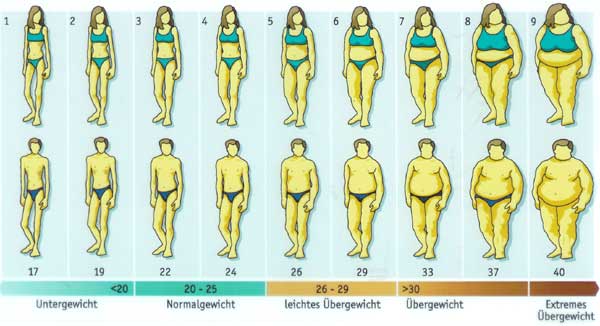
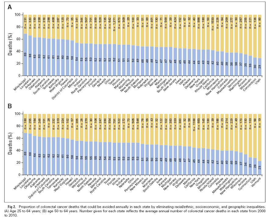
My question is: if BMI already accounts for stature, then why would there different cut-points for Asian sub-populations? One might answer: “Because at a given BMI, Asians have a higher diabetes risk than non-Hispanic Whites.” But if that is the justification, then shouldn't we also have a lower cut-point for poor people? Moreover, the WHO cut-points were recommended for Asians, not for Asian-Americans. We know from decades of research that immigrants take on the risk profile of their adopted countries. So how many generations would it take for Asian-Americans to get the American cut-points instead of the Asian cut-points? Obviously the application of the Asian threshold to people born in the US turns a regional norm into a racial trait. The authors write "In particular, we focused on prevalence of diabetes in the category 23–24.9 kg/m2, in which Asians are considered overweight by the WHO guidelines while non-Asians are not, and in the category 27.5–29.9 kg/m2, in which Asians are considered obese but the other the groups are classified as overweight." Do these folks know what a BMI of 23 kg/m2 looks like? If someone thinks that women 3 and 4 below are "overweight", I think they may have a perceptual disorder. The authors of this paper calculated age-standardized colorectal cancer death rates for three education categories by race/ethnicity and state among individuals age 25 to 64 years from 2008 through 2010.
They then calculated the proportion of premature death resulting from colorectal cancer that could potentially be averted in each state by applying the average death rate for the five states with the lowest rates among the most educated whites (Connecticut, North Dakota, Utah, Vermont, and Wisconsin) to all populations. Education had a big effect for blacks and whites in almost all states, but the authors concluded that half the premature deaths resulting from colorectal cancer that occurred nationwide from 2008 through 2010, or 7,690 deaths annually, would have been avoided if everyone had experienced the lowest death rates of the most educated whites. More premature deaths could have been avoided in southern states (60-70%) than in northern and western states (30-40%). This article by David Tuller in the New York Times (February 27, 2015) reports on the discovery of a biomarker for chronic fatigue syndrome, which apparently is no longer called chronic fatigue syndrome. The story reports that the Institute of Medicine has changed the name of this condition to “systemic exertion intolerance disease”, which I interpret as an attempt to make it sound more like a real disease that could be treated pharmaceutically, and less like a label for lazy people. Anyway, the scientists speculate that this could form the basis for the first clinical diagnosis for the illness. The research article was published in the new open access journal Science Advances, which critics have assailed not only because of unprecedented high publication fees (more than $5000 per article) but also because it turns out to not really be open access after all.
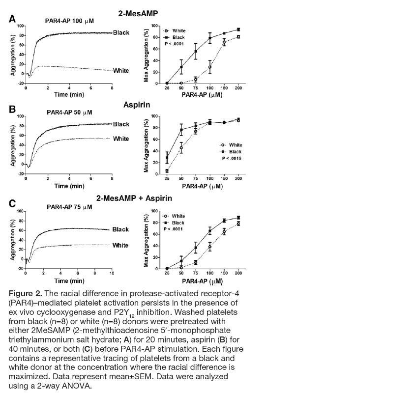
But the real point of this post is to note the shockingly frank description of p-hacking in the news report. These authors seem to have no shame about this, which I suspect means that they don't really know that they did anything wrong. Neither, apparently, do the reviewers of Science Advances. Here is how the New York Times describes the analysis in the paper: "For the study, the research team — which included scientists from Columbia, Stanford and Harvard — tested the blood of 298 patients with the syndrome, and 348 healthy people who served as a control group, for 51 cytokines, substances that function as messengers for the immune system. When the team compared all the patients with all the healthy controls, they found no significant differences between the two groups. But after dividing the patients into two cohorts — those who had been sick for less than three years and those who had been sick longer — they found sharp differences. And both sets of patients were different from healthy controls." They don't mention how many cut-points they tried before they came up with 3 years. Any bets on whether this one holds up or not? While we're looking at this one, here's a line from the paper that impressed me on page 3: "Two proinflammatory cytokines had a prominent association with short-duration ME/CFS (Table 2). This association was markedly elevated for interferon-g (IFNg), with an OR of 104.77 (95% CI, 6.975 to 1574.021; P = 0.001)." That's an impressively wide interval. And I confess that I was a bit baffled by this bit of text on page 8: "GLM analyses were applied to examine both the main effect of diagnosis and the main and interaction effects of different fixed factors including diagnosis (two-level case versus control comparisons and three-level short duration versus long duration versus control analyses) and sex, with age adjusted as a continuous covariate. Because GLM uses the family-wise error rate, no additional adjustments for multiple comparisons were applied." So you can't be accused of p-hacking if you fit a GLM because it fits a "family-wise error rate"? I have no idea what their talking about there, but maybe that's my problem, not theirs. In this study, authors recruited 19 white volunteers (mean age 31.9 ± 1.8) and 28 black volunteers (mean age 40.4 ± 2.4) and with no adjustments for age or any other relevant factors (e.g. diet, obesity, co-morbidity, physical activity, prescriptions, socioeconomic status, etc) concluded that
"[o]ur study is the first to demonstrate that the Gq pathway is differentially regulated by race." (abstract). Despite the small numbers, the authors also further restricted by factors that could similarly be affected by age, diet, comorbidity or other unmeasured characteristics distributed differentially by race: "To determine whether potential differences exist in the kinetics of platelet activation, the time to 50% aggregation was measured, which encompasses both the lag time (the time from agonist addition until the start of aggregation) as well as the rate of aggregation. Because not all donors aggregated in response to threshold doses of PAR4-AP, platelets from subjects who failed to reach 50% aggregation were eliminated from the analysis. For the donors who did not reach 50% aggregation, 6 of 13 white donors at 35 μmol/L of PAR4-AP and 3 of 12 white donors at 50 μmol/L of PAR4-AP were excluded from the analysis. Even with the absence of several white subjects because of lack of platelet aggregation, platelets from white donors were slower to 50% aggregation compared with platelets from black donors at low concentrations of PAR4-AP (35–50 μmol/L; Figure 1H). These data suggest that the racial difference in PAR4-mediated platelet activation is intrinsic to the platelet." (p. 2646) The journal Arteriosclerosis, Thrombosis, and Vascular Biology, is an American Heart Association journal that is considered pretty reputable, or so I thought. This news story on inhabitat.com reports on Bill H.R. 1422 (the Science Advisory Board Reform Act):
House Passes Bill That Prohibits Expert Scientific Advice to the EPA By Beverley Mitchell, Inhabitat 25 February 15 While everyone’s attention was focused on the Senate and the Keystone XL decision on Tuesday, some pretty shocking stuff was quietly going on in the House of Representatives. The GOP-dominated House passed a bill that effectively prevents scientists who are peer-reviewed experts in their field from providing advice — directly or indirectly — to the EPA, while at the same time allowing industry representatives with financial interests in fossil fuels to have their say. Perversely, all this is being done in the name of “transparency.” Bill H.R. 1422, also known as the Science Advisory Board Reform Act, passed 229-191. It was sponsored by Representative Chris Stewart (R-UT). The bill changes the rules for appointing members to the Science Advisory Board (SAB), which provides scientific advice to the EPA Administrator. Among many other things, it states: “Board members may not participate in advisory activities that directly or indirectly involve review or evaluation of their own work.” This means that a scientist who had published a peer-reviewed paper on a particular topic would not be able to advise the EPA on the findings contained within that paper. That is, the very scientists who know the subject matter best would not be able to discuss it. On Monday, the White House issued a statement indicating it would veto the bill if it passed, noting: “H.R. 1422 would negatively affect the appointment of experts and would weaken the scientific independence and integrity of the SAB.” Representative Jim McGovern (D-MA) was more blunt, telling House Republicans on Tuesday: “I get it, you don’t like science. And you don’t like science that interferes with the interests of your corporate clients. But we need science to protect public health and the environment.” Director of the Union of Concerned Scientists Andrew A. Rosenberg wrote a letter to House Representatives stating: “This [bill] effectively turns the idea of conflict of interest on its head, with the bizarre presumption that corporate experts with direct financial interests are not conflicted while academics who work on these issues are. Of course, a scientist with expertise on topics the Science Advisory Board addresses likely will have done peer-reviewed studies on that topic. That makes the scientist’s evaluation more valuable, not less.” Two more bills relating to the EPA are set to go to the vote this week, bills that opponents argue are part of an “unrelenting partisan attack” on the EPA and that demonstrate more support for industrial polluters than the public health concerns of the American people. This press release, reporting on this article, reveals that "Increasing diet soda intake is directly linked to greater abdominal obesity in adults 65 years of age and older." I think that the adjective "directly" is meant to specify that the correlation is positive, but it could be confused to imply the absence of mediators.
In any case, the importance of this correlation is described as follows: "Findings raise concerns about the safety of chronic diet soda consumption, which may increase belly fat and contribute to greater risk of metabolic syndrome and cardiovascular diseases." Moreover, the authors recommend that "older individuals who drink diet soda daily, particularly those at high cardiometabolic risk, should try to curb their consumption of artificially sweetened drinks." The authors are proposing that diet soda makes people fatter. The obvious alternative hypothesis, which seems substantially more plausible to me, is that people who are gaining weight drink more diet soda as an attempt to mitigate this trend. It could even be that this strategy is successful, and that without diet soda, they would have gained even more weight. The authors measured reported diet soda consumption and anthropometrics simultaneously at each follow-up wave of the study, and no lags were employed to account for this possibility of reverse causation. To their credit, in the "limitations" section of the paper, the authors do question this association: "Whether [diet soda index] exacerbated the [waist circumference] gains observed in SALSA participants is unclear; the analyses include adjustment for anthropometric measures and other characteristics at the outset of each follow-up interval, but other factors—including family history and perceived personal weight-gain and health-risk trajectories —that increased [change in waist circumference] but were not captured in the analyses may have influenced participant decisions to use [diet soda]." But the adjustment for baseline doesn't solve the potential reverse causation here because baseline anthropometrics are measured at the same time as soda consumption. And in any case, this doubt about the interpretation of the effect is completely lost by the time the authors reach the conclusion section, and no caveats whatsoever are expressed in the press release, which ends with the recommendation to curb consumption of artificially sweetened drinks. They don't specify what people should be drinking instead. In the April 11 2015 issue of The Lancet, Richard Horton asks what we can do about the fact that “A lot of what is published is incorrect.” As a solution, Horton suggests a p-value criterion for "significance" of 10 to the -7. But in genetic epidemiology they already use something around 10 to the -7 and the results in that field are even less reproducible than the rest of epidemiology! No, clearly we need to go in the other direction and get rid of null hypothesis significance testing altogether. Rather, as eluded to earlier in the essay, we need to change the incentive structure so that one doesn't get rewarded for being published, but instead one gets rewarded for being right. Suppose that if your result were shown to be wrong, you had to give back the grant money. Then you'd see people checking for errors! In engineering, if your bridge falls down or your airplane crashes, you are gonna get fired. But do you see Walt Willett getting fired for the epidemiologic equivalent? Changing the p-value criterion before you can declare something to be "significant" is not going to help this problem.
This press release about this article considers gene by environment (childhood abuse) interactions contributing to the risk of depression. The authors analysed a sample of 2679 Spanish primary care patients ages 18 to 75. The paper reports that those who have low functioning alleles in functional genes for neurotrophism (BDNF) and serotonin transmission are particularly vulnerable to the effects of childhood abuse (psychological, physical or sexual) as a risk factor for clinical depression. They also included an additional level of interaction with treatment, taking into account the response to antidepressants.
I am sceptical about the statistical power necessary for testing 3-way interactions among 2679 subjects, not to mention the use of odds ratios for common outcomes. But my biggest gripe is that they tested for synergism by looking at the p-value for the product interaction term in a logistic regression model, which detects deviation from multiplicativity. Deviation from additivity is really what they want here. In fact, their estimates are mostly greater than multiplicative, and therefore there is no doubt about them being synergistic. But it presents an incorrect method for making this G x E interaction analysis. Not to mention that they exponentiate the interaction term coefficient and call that an odds ratio. It would be better of course to use a measure like RERI to detect greater than additive joint effects between genotype and abuse history, but since the outcome is not rare, it is also better to rely on the RR rather than the OR in making that calculation, as noted by Kalilani and Atashili 2006. This news story reports on this new article about smoking, obesity and genotype. The variant of interest, which causes smokers to smoke more heavily, was associated with increased BMI, but only in those who have never smoked. This seemed at first a surprising and intriguing new result, and the press release makes it sound really exciting as a paradigm for GxE interactions. All good.
Except that when I went to read the article I found that the estimated effect of this SNP in CHRNA5-A3-B4 is to reduce BMI by a whopping 0.74%. I'll bet that less than 1% of your BMI is around an amount of weight that you gain or lose over the course of a meal. The same SNP caused 0.35% higher BMI in never smokers, an effect half as large, and I seriously doubt that a third of a percent of a BMI point is even within the measurement error of the scales they used in the study (and certainly less than the normal weight variation across a typical day). The p-values here are small because the study is so enormous, but the effect sizes are so absurdly trivial that this could never have any observable impact on an individual level. To be fair, if the estimated effect were huge, it would be implausible, so this is a finding that could really be true. By aside from what it might reveal about the underlying biology, it seems irrelevant. Moreover, when effects are this small, the tiniest violation (e.g. of their exclusion restriction assumption for their Mendelian randomization) could easily dwarf the claimed result. Not something that Sandro Galea could call “consequential epidemiology”, I don’t think. I like the idea of GxE in principle, since the world must work this way. But if effects are in this range, which seems realistic, then it doesn’t seem that we can have a lot of confidence in the results (i.e. it wouldn’t take very much bias to knock you off center by a third of a percent), and even if true, the results wouldn’t have any direct implications for either population or individual health. I guess if we accumulated enough such examples, it could start to make a meaningful difference in phenotype. Maybe we’re just at the beginning of a long process of knowledge accumulation. |
 RSS Feed