We all know that the change in estimate approach to finding confounders can't work for the OR because the OR can change its value when conditioned on any determinant of outcome, even if the covariate is independent of exposure. Therefore, the OR will "cry-wolf" and claim confounders that aren't confounders (when they are not associated with exposure). It can also fail to detect a true confounder, although a recent paper by Mansournia and Greenland notes that this is decidedly less likely to occur, because it requires an incidental canceling out. On the other hand, the false accusation of confounders by a change in estimate approach applied to an OR is quite easy to encounter. This will happen whenever the frequency of the outcome is high in the data set.
Here is a quick Stata example that generates a data set of binary variables:
clear all
set obs 10000
set seed 12345
gen c = rnormal()
gen x = rnormal()
gen y = rnormal() + x + c
replace c = (c > 0)
replace x = (x > 0)
replace y = (y > 0)
This code generates a binary Y that is a function of both exposure X and covariate C.
X and C are completely independent (ORXC = 1). Therefore C by definition cannot be a confounder. Prevalence of Y=1 is 0.5.
logistic y x
logistic y x c
Crude ORYX = 5
When I adjust this for C, I get ORYX|C = 7.
Therefore, by change in estimate criteria, one might think that they have to adjust for C. But this is wrong. The OR is "crying wolf".
So far so good. We also know that the RD is collapsible, and sure enough:
binreg y x, rd
binreg y x c, rd
Crude RDYX = 0.38
When I adjust this for C, I get RDYX|C = 0.38.
Therefore, by change in estimate criteria, one would not adjust for C, which is the right answer. Good.
But here is the surprise:
binreg y x, rr
binreg y x c, rr
Crude RRYX = 2.30
When I adjust this for C, I get RRYX|C = 2.08.
These are significantly different, and therefore, by change in estimate criteria, one might adjust for C, which would be a mistake.
The RR is supposed to be collapsible, so this baffled me until I looked at the stratum specific estimates:
cs y x, by(c)
cs y x, by(c) istandard
cs y x, by(c) estandard
c | RR [95% CI]
-----------------+-------------------------------------
0 | 4.54 4.04, 5.11
1 | 1.75 1.68, 1.83
-----------------+-------------------------------------
Crude | 2.30 2.19, 2.40
M-H combined | 2.26 2.16, 2.36
I. Standardized | 2.24 2.15, 2.34
E. Standardized | 2.27 2.18, 2.37
For those of you who don't know Stata, "internally standardized" is standardization using the X=1 group as the target population, and "externally standardized" is standardization using the X=0 group as the target population (old occupational health terminology). X and C are uncorrelated in expectation, so these target-population-specific adjusted values differ only due to the chance imbalance in C across levels of X.
So there is tremendous effect modification by C here, even though C is not a confounder. This doesn't seem to matter for the RD, but for the RR, getting the right answer seems to depend on exactly HOW I adjust for C. These standardized estimates are slightly different, but they are all statistically homogeneous with the crude. But the binomial regression adjusted estimate is much lower than the standardized estimates (RR = 2.09). If I use Poisson regression, I get RR=2.26, so again it is collapsible, so it seems that only the binomial regression estimate is screwy here. Should one avoid binomial regression when the outcome is common or the effect of the exposure is heterogeneous?
I was sincerely confused, so I sent e-mail around to some friends, and after some discussion, it all seemed quite obvious.
My Stata code generates the following (true) proportions of Y=1 in each stratum of X and C:
. table x c, c(mean y)
------------------------------
| c
x | 0 1
----------+-------------------
0 | 0.1084666 0.5012356
1 | 0.4927478 0.8789078
------------------------------
Logistic regression:
------------------------------
| c
x | 0 1
----------+-------------------
0 | 0.112023 0.4974815
1 | 0.4890754 0.8825148
------------------------------
Binomial regression:
------------------------------
| c
x | 0 1
----------+-------------------
0 | 0.2031814 0.4296737
1 | 0.4217731 0.8919361
------------------------------
Poisson regression:
------------------------------
| c
x | 0 1
----------+-------------------
0 | 0.1835052 0.4220249
1 | 0.4152605 0.9550153
------------------------------
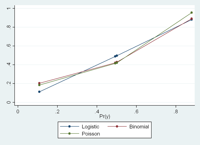
Logistic is not perfect here, but much better than the other two. Still, it is not that logistic is somehow superior in any general sense for this task. It just got lucky in this instance.
The two stratum-specific ORs are 8.0 and 7.2, which happen to be much closer to being homogeneous than the two true RR’s (4.5 and 1.8). The fact that the two true RDs are roughly homogeneous (0.38 and 0.38) explains why the additive model does so well.
As Rich MacLehose kindly pointed out, this has nothing to do with collapsibility, per se. It has to do with model fit. If the model is misspecified, you can easily get change in estimate that suggests confounding, regardless of the choice of effect estimate. In *ALL* of these models, when I add an interaction term, I get the exactly correct predicted proportions in every cell, and the correct RRs or ORs when I divide these predictions. So the moral of the story is that change in estimate is not a sufficient criterion, even with a collapsible measure. One also has to get the model right. Seems obvious in retrospect, but in practice, how often do we worry about this? The well-known Greenland and Morgenstern example shows RR collapsibility even when the stratum specific RRs are very heterogeneous, but they use tabular (i.e. non-parametric) adjustments In their example, if one used a regression model, one would not generally reach the same conclusion (without adding interaction terms).
But Rich also asked another question, which is how it can be that Poisson Regression and Binomial Regression produce different point estimates when they have the same link function and differ only in the error distribution.
I also hadn't previously thought in detail about this, and if students asked I probably would have answered the same: that changing the distribution in the GLM would affect the CIs but not the point estimates. But I think that my (bad) intuition stems from equating rates and risks. If the outcome were rare, I think we would indeed see that these give approximately the same value. But the problem is that the outcome in my example is common, and in some cells VERY common. That apparently messes things up. Specifically, logistic model searches for the best (ML) solution under the constraint that all the log-odds fall on a straight line. Binomial regression searches for the best (ML) solution under the constraint that all the log-risks fall on a straight line. Poisson searches for the best (ML) solution under the constraint that all the log-rates fall on a straight line. So I guess what we are seeing here is the distinction between risks and rates. The surprising thing about that is that I have no person time here (no offset in the Poisson model), so everyone has 1 time unit, so I can't see how the rate and risk could be different. So that remains a bit of a mystery for me.
If you look at a plot of the fitted values for the three models (truth versus logistic, binomial and Poisson), you see that logistic comes closest in this instance because the true proportions are closest to being linear in the log odds than to any of the other scales:
Here is a quick Stata example that generates a data set of binary variables:
clear all
set obs 10000
set seed 12345
gen c = rnormal()
gen x = rnormal()
gen y = rnormal() + x + c
replace c = (c > 0)
replace x = (x > 0)
replace y = (y > 0)
This code generates a binary Y that is a function of both exposure X and covariate C.
X and C are completely independent (ORXC = 1). Therefore C by definition cannot be a confounder. Prevalence of Y=1 is 0.5.
logistic y x
logistic y x c
Crude ORYX = 5
When I adjust this for C, I get ORYX|C = 7.
Therefore, by change in estimate criteria, one might think that they have to adjust for C. But this is wrong. The OR is "crying wolf".
So far so good. We also know that the RD is collapsible, and sure enough:
binreg y x, rd
binreg y x c, rd
Crude RDYX = 0.38
When I adjust this for C, I get RDYX|C = 0.38.
Therefore, by change in estimate criteria, one would not adjust for C, which is the right answer. Good.
But here is the surprise:
binreg y x, rr
binreg y x c, rr
Crude RRYX = 2.30
When I adjust this for C, I get RRYX|C = 2.08.
These are significantly different, and therefore, by change in estimate criteria, one might adjust for C, which would be a mistake.
The RR is supposed to be collapsible, so this baffled me until I looked at the stratum specific estimates:
cs y x, by(c)
cs y x, by(c) istandard
cs y x, by(c) estandard
c | RR [95% CI]
-----------------+-------------------------------------
0 | 4.54 4.04, 5.11
1 | 1.75 1.68, 1.83
-----------------+-------------------------------------
Crude | 2.30 2.19, 2.40
M-H combined | 2.26 2.16, 2.36
I. Standardized | 2.24 2.15, 2.34
E. Standardized | 2.27 2.18, 2.37
For those of you who don't know Stata, "internally standardized" is standardization using the X=1 group as the target population, and "externally standardized" is standardization using the X=0 group as the target population (old occupational health terminology). X and C are uncorrelated in expectation, so these target-population-specific adjusted values differ only due to the chance imbalance in C across levels of X.
So there is tremendous effect modification by C here, even though C is not a confounder. This doesn't seem to matter for the RD, but for the RR, getting the right answer seems to depend on exactly HOW I adjust for C. These standardized estimates are slightly different, but they are all statistically homogeneous with the crude. But the binomial regression adjusted estimate is much lower than the standardized estimates (RR = 2.09). If I use Poisson regression, I get RR=2.26, so again it is collapsible, so it seems that only the binomial regression estimate is screwy here. Should one avoid binomial regression when the outcome is common or the effect of the exposure is heterogeneous?
I was sincerely confused, so I sent e-mail around to some friends, and after some discussion, it all seemed quite obvious.
My Stata code generates the following (true) proportions of Y=1 in each stratum of X and C:
. table x c, c(mean y)
------------------------------
| c
x | 0 1
----------+-------------------
0 | 0.1084666 0.5012356
1 | 0.4927478 0.8789078
------------------------------
Logistic regression:
------------------------------
| c
x | 0 1
----------+-------------------
0 | 0.112023 0.4974815
1 | 0.4890754 0.8825148
------------------------------
Binomial regression:
------------------------------
| c
x | 0 1
----------+-------------------
0 | 0.2031814 0.4296737
1 | 0.4217731 0.8919361
------------------------------
Poisson regression:
------------------------------
| c
x | 0 1
----------+-------------------
0 | 0.1835052 0.4220249
1 | 0.4152605 0.9550153
------------------------------
Logistic is not perfect here, but much better than the other two. Still, it is not that logistic is somehow superior in any general sense for this task. It just got lucky in this instance.
The two stratum-specific ORs are 8.0 and 7.2, which happen to be much closer to being homogeneous than the two true RR’s (4.5 and 1.8). The fact that the two true RDs are roughly homogeneous (0.38 and 0.38) explains why the additive model does so well.
As Rich MacLehose kindly pointed out, this has nothing to do with collapsibility, per se. It has to do with model fit. If the model is misspecified, you can easily get change in estimate that suggests confounding, regardless of the choice of effect estimate. In *ALL* of these models, when I add an interaction term, I get the exactly correct predicted proportions in every cell, and the correct RRs or ORs when I divide these predictions. So the moral of the story is that change in estimate is not a sufficient criterion, even with a collapsible measure. One also has to get the model right. Seems obvious in retrospect, but in practice, how often do we worry about this? The well-known Greenland and Morgenstern example shows RR collapsibility even when the stratum specific RRs are very heterogeneous, but they use tabular (i.e. non-parametric) adjustments In their example, if one used a regression model, one would not generally reach the same conclusion (without adding interaction terms).
But Rich also asked another question, which is how it can be that Poisson Regression and Binomial Regression produce different point estimates when they have the same link function and differ only in the error distribution.
I also hadn't previously thought in detail about this, and if students asked I probably would have answered the same: that changing the distribution in the GLM would affect the CIs but not the point estimates. But I think that my (bad) intuition stems from equating rates and risks. If the outcome were rare, I think we would indeed see that these give approximately the same value. But the problem is that the outcome in my example is common, and in some cells VERY common. That apparently messes things up. Specifically, logistic model searches for the best (ML) solution under the constraint that all the log-odds fall on a straight line. Binomial regression searches for the best (ML) solution under the constraint that all the log-risks fall on a straight line. Poisson searches for the best (ML) solution under the constraint that all the log-rates fall on a straight line. So I guess what we are seeing here is the distinction between risks and rates. The surprising thing about that is that I have no person time here (no offset in the Poisson model), so everyone has 1 time unit, so I can't see how the rate and risk could be different. So that remains a bit of a mystery for me.
If you look at a plot of the fitted values for the three models (truth versus logistic, binomial and Poisson), you see that logistic comes closest in this instance because the true proportions are closest to being linear in the log odds than to any of the other scales:
But even though Binomial and Poisson match almost exactly on the low end, they diverge markedly at the high end. This makes me think that we could see the distinction much more clearly if we don't convert everything to binary variables. So I ran this again with continuous x and c:
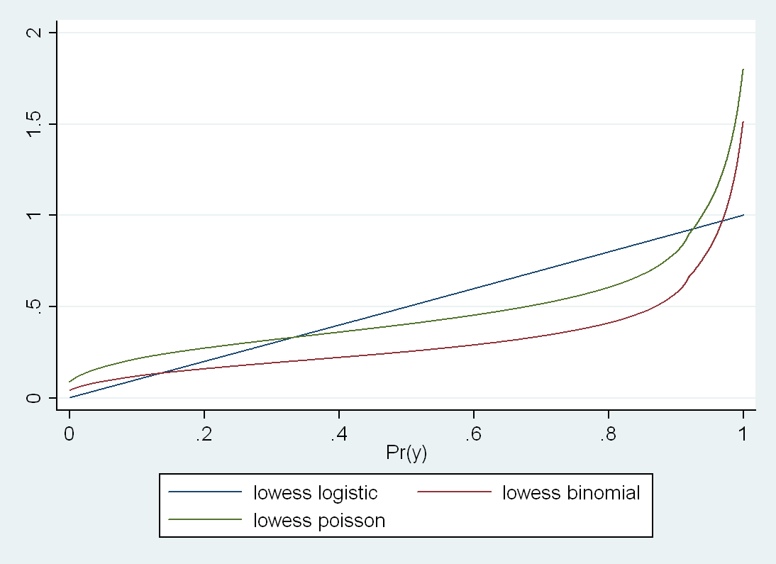
I had a hard time getting binomial regression to converge, and ended up having to plot this with a smoother because the predicted line was jagged for binomial because of the difficulty in obtaining convergence. But in any case, now one can see that the shape of the underlying function is rather different between Poisson and Binomial here. If you don't smooth, Poisson shoots up
much more dramatically at the upper limit as you get very close to 1 in the true probability. Even on the low end they are not that close, but I think that this is because the model is trying to find the ML solution that also works on the top end.
And bear in mind that the logistic looks straight here only because the data in my particular example happened to be approximately homogeneous in the ORs across strata of C, but one could engineer an example where logistic would do very poorly, too.
Moral of the story: use interaction terms to make a saturated model, and then use –margins- to take the differences or ratios of the correctly specified risks (what Sam Harper recommended to me from the start). Common wisdom that Poisson and Binomial are estimating the same parameter comes from a rare outcome setting. When the outcome is not rare, these are not going to agree, and there is no way to predict which will be closer to the truth in any given instance.
Again, all this seems obvious in retrospect, but then again, most things do.
 RSS Feed